Coronavirus - Uncertainty in Case Estimates

I have no knowledge of epidemiology. Everything below is deeply suspect. This is very much a work in progress.

I’m intentionally leaving the exposition here fairly bare-bones, and the results ugly and messily presented, because I don’t want e.g. a nice pretty results plot to be shared to someone who doesn’t understand that the results are deeply suspect because they come from a deeply suspect model. I’m a little worried about beautiful shiny plots from stats people with no background in infectious disease being taken too seriously by non-specialists.

Caveats over.

Initial Motivation

We’re interested in how the true covid-19 case count is developing over time – in particular, we’d like to estimate the total current case count. There are some major complications to getting this case count, three of which are:

1. There’s an incubation period, during which infections wouldn’t be visible even if we had perfect observations of symptomatic cases.
2. There’s a delay between symptoms appearing and getting a confirmed diagnosis.
3. Not all cases will be observed for many reasons, e.g. very mild symptoms, lack of testing, etc.

I’ve seen a couple of back-of-the-envelope calculations using average numbers for points 1 and/or 2 above. I think that it’s important to take account of the full probability distribution for 1 and 2, because the tails are potentially very important. A small proportion of cases with a long incubation period would mean a small increase in our estimate for how many people were infected earlier on. Given the exponential growth of infections, a few extra infections earlier on might make a big difference to the current case count. Dealing with this issue was my motivation for starting this work. As a bonus, we can get not just a point estimate for the current number of cases, but a probability distribution – ideally this will meaningfully quantify our uncertainty. We’re going to get this distribution by setting up a model for how the observed confirmed case counts depend on the unobserved true case counts, and feeding this model into a probabilistic programming language to do approximate MCMC inference.

What can we do about each of these issues above?

1. As of 10/03/2020, researchers at Johns Hopkins give a log-normal distribution for the incubation period in days, with $\mu = 1.621$, $\sigma = 0.418$ for the underlying normal in log space¹.
2. I hope there is some data out there for this, since it seems like the sort of thing that healthcare workers would be able to collect (“when did you first notice your symptoms?” seems like a normal question to ask patients), but I don’t have any data right now. We’ll do the best we can but an actual estimate for this distribution would be very helpful. I’d expect this to vary enormously by country.
3. We might not be able to deal with point 3 very well, but we can maybe do something about it by incorporating fatality data, because we expect fatalities to be much more comprehensively observed. We’ll come back to this point later.

First steps to the model

For the basic setup, first assume that everyone becomes a confirmed case on the day they become symptomatic. i.e. we’re first going to worry only about issue 1 from above. We’ll fix this shortly but it’s easier to think about things this way to begin with. Let’s set up some notation:

• Let $t=0$ stand for today, $t=-1$ yesterday, and so on.
• Write $x_t$ for the total number of confirmed people by day $t$.
• Write $z_t$ for the number of people who became newly infected on day $t$ and will eventually get a confirmed diagnosis.
  • So here $x_t$ is cumulative, and $z_t$ is not.
  • We’re most interested in $z_0$, the new infections that happened today. We can work back from this to get the cumulative total.
    • We will need to scale this up at some point to deal with totally unobserved cases.
• Let $q^i_s$ (for in-q-bation period, I guess…) be the number of days that the $i$-th infected person on day $s$ takes to become symptomatic.
• Write $S^i_{s,t}$ for the event that the $i$-th infected person on day $s$ is symptomatic on or before day $t$.

Then we have $S^i_{s,t} = 0$ if $q > t - s$, $S^i_{s,t} = 1$ if $q \leq t - s$.

These definitions give us an expression for the observed cumulative count $x_t$ in terms of the unobserved daily counts $z_s$:

\[x_t = \sum_{s = -\infty}^t \sum_{i=1}^{z_s} S^i_{s, t}\]

Now let’s regard the $q^i_s$ as being drawn i.i.d. from our lognormal distribution for the incubation period. Then the $S^i_{s, t}$ are identically distributed Bernoulli random variables, and for a fixed value of $t$ they’re also independent. A sum of Bernoullis is binomial, so this gives us $x_t$ as a sum of binomial random variables.

Our goal now is to get a posterior distribution for $z_0$, and for that we’ll need need a prior. The growth of $z_s$ over time is probably close enough to exponential right now that we don’t lose that much by assuming it’s exactly exponential, and it simplifies the model considerably to do so. We’ll put a broad log-normal prior on $z_0$ and a uniform $[1, 1.5]$ prior on the base of the exponential, $r$. NB The prior for $\mu$ should vary drastically depending on the day the region you’re trying to model.

Dealing with the lag between symptom onset and diagnosis

For now we can’t do much better than take a total guess at this. We probably expect that not many people get diagnosed in the first couple of days after showing symptoms, there’s a peak after a few days, and then it tails off again. It’ll look a little bit like a Poisson distribution. That’s a totally inappropriate distribution but we’ll go with it for now because it’s vaguely the right shape.² When we code up the model, we’ll put a broad Gamma prior over the parameter to this Poisson distribution. We’ll call this parameter $\lambda$.

Incorporating this delay will be reasonably straightforward if we simplify our distribution for $x_t$ a little, so let’s do that.

Simplifying the model

We’ve noted that the sum $\sum_{i=1}^{z_s} S_{s,t}^i$ is a binomial distribution. Writing $\pi$ for the CDF of our incubation period distribution, the parameters are $n = z_s$ and $p = \pi(t-s)$. We can approximate this by a Poisson distribution with $\lambda_{st} = z_s \pi(t-s)$.

So we now have $x_t$ as a sum of Poisson variables:

\[x_t = \sum_{s = -\infty}^t \text{Pois}(\lambda_{st})\]

These Poissons are independent, since all the $S^i_{s,t}$ were independent. But the sum of independent Poisson random variables is Poisson. We thus have:

\[x_t \sim \text{Pois}\left(\sum_{s=-\infty}^t \lambda_{st} \right)\]

Let $\mu_t = \sum_{s=-\infty}^t \lambda_{st}$, so:

\[x_t \sim \text{Pois}\left(\mu_t\right)\]

We know that the $x_t$ aren’t independent across different values of $t$. The following transformation leaves the marginal distribution of $x_t$ intact but gets rid of the independence assumption:

\[x_{t+1} = x_t + \text{Pois}\left(\mu_{t+1} - \mu_t\right)\]

The Poissons here are independent. This at least means that the marginal distribution of each $x_t$ is still correct, and it enforces that $x_t$ is monotonically increasing in $t$. I suspect this isn’t right but we’ll go with it for now. We’ll need to look back in time to some initial $x_{-T} \sim \text{Pois}(\mu_{-T})$.

Now how can we incorporate the $\text{Pois}(\lambda)$ delay between symptom onset and diagnosis that we introduced above? We have to add an independent $\text{Pois}(\lambda)$ to each $q$ above. This means we’re counting the time spent waiting to get a confirmed diagnosis as part of the overall “infection to confirmation” incubation period. $S^i_{s,t}$ are still iid Bernoulli, but our $p$ for that Bernoulli has changed. Above, that $p$ was just $\pi(t-s)$, where $\pi$ is the CDF for the incubation period. We now need the CDF for the combined waiting period. We’ll denote this $c$.

Writing $P$ for the probability mass function of our $\text{Pois}(\lambda)$, the required CDF is:

\[c(x) = \sum_{i=0}^\infty P(i) \pi (x-i)\]

The $p$ in our Bernoulli is no longer $\pi(t-s)$ as above, but $c(t-s)$. We can run through exactly the same binomial-to-Poisson argument as above and redefined our $\mu_t$ appropriately to take into account the extra waiting time.

If we can find out the true empirical distribution of the time between symptom onset and confirmed test result, we can sub that in for $P$, get rid of a free parameter and ideally get better results.

Incorporating death rate

We expect deaths to be observed much more comprehensively than infections, so incorporating fatality counts might let us estimate how badly the confirmed cases undercount the real cases. That assumes that we somehow have a reasonable estimate of the true fatality rate from somewhere else – this is one serious weak point among many for this model.

For notation, we’ll denote the total number of deaths on or before day $t$ by $y_t$.

Similarly to our view of the incubation time, we’re going to take a probabilistic view on the length of time between symptom onset and death. This paper from the Journal of Clinical Medicine³ gives a log-normal distribution for the time from symptom onset to death, with $(\mu=2.83, \sigma=0.59)$. Write $D^i_{s,t}$ for the event that the $i$-th person infected on day $s$ is dead on or before day $t$. Let’s assume a 1% death rate.

By similar reasoning to the above we’ll get a Poisson distribution for $y_t$.⁴ As above, the parameter for this Poisson will depend on some CDF. In this case, it’s the CDF for the sum of the incubation period and the time from symptom onset to death. This is a sum of two log-normals. There’s no closed-form CDF for this, so we’ll approximate the sum as another log-normal with the correct mean and variance⁵. Write $\phi$ for this cdf.

One more difference from last time is that we need to take into account the fact that $z_s$ undercounts the true cases. We’ll assume that this undercounting is a constant factor, and we’ll denote that factor $K$. That’s one more free parameter for the model.

So this time, $\lambda_{st} = K z_s \phi(t - s)$, and we’ll have to divide through by 100 for the death rate. So:

\[100 y_t = \text{Pois}\left(K \sum_{s=-\infty}^t z_s \phi(t - s) \right)\]

Again we should worry about the fact that these are not independent, so exactly as for the expression for $x_t$, we’ll set $\nu_t = K \sum_{s=-\infty}^t z_s \phi(t - s)$ and say:

\[100 y_{t+1} = 100 y_t + \text{Pois}\left(\nu_{t+1} - \nu_t\right)\]

To be clear, at this point we’re saying $z_t$ is “number who became infected on day $t$ and will eventually get a diagnosis”, and “true number who became infected” is therefore $K z_t$.

Code

I’ve implemented this model as a probabilistic program in pyStan. Code for the model is available here. NB In the code, time is indexed backwards, since it was a bit simpler to implement things this way. So $t=1$ is yesterday, and so on…

Preliminary Results

These results come from a run of the model with 4 chains of 10,000 samples each.

• Assumed fatality rate 1%
• $\mu = \text{log}(4000), \sigma = 4$ for the prior on $z_0$.
• $\text{Gamma}(1.5, 0.1)$ prior on the parameter $\lambda$ of the Poisson distribution governing symptom-to-confirmation lag.
• Uniform $[1, 1000]$ prior on the ratio $K$ of total cases to cases which will never be diagnosed.
  • Yes, this seems insanely wide. I initially tried $[1, 10]$, and the model didn’t constrain $K$ well but said it was more likely to be at the higher and of that range. Then tried $[1, 100]$ to give it more space at the upper end, and it was reasonably close to uniform on that interval. So I widened it again to see if the model would just accept any value whatsoever for $K$. It does constrain it to the sub-$100$ range with this very broad prior.
• Case and fatality data is for the UK as of Sunday 15th March, so $K z_0$ is our estimate for the number of newly infected people that day.

Plots are ugly because I’m using unfamiliar tools in a hurry and for reasons mentioned above.

These results show estimates for 5 things:

1. $z_0$, the number of new cases today which will eventually be confirmed cases.
2. $K$, the factor by which $z_0$ underestimates the true case count (because some will never be confirmed).
3. $K z_0$, the true number of new cases today.
4. $\lambda$, a parameter governing how long it takes to obtain a confirmed diagnosis after becoming symptomatic.
5. $r$, the daily rate of increase in infections.

Here’s the posterior for $K z_0$:

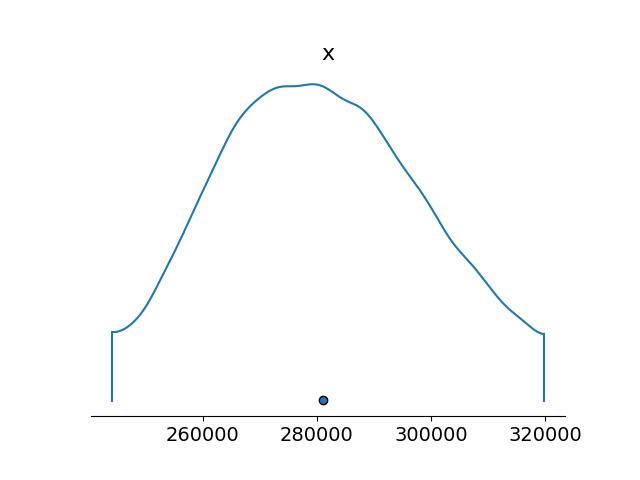
Standard deviation for this is about $20,000$.

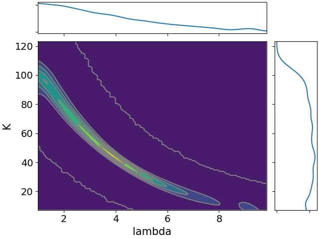
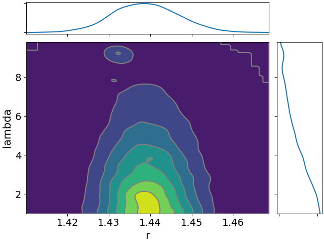
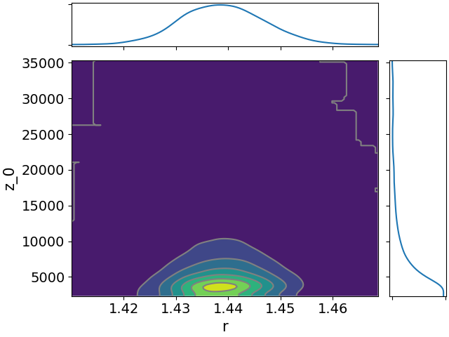
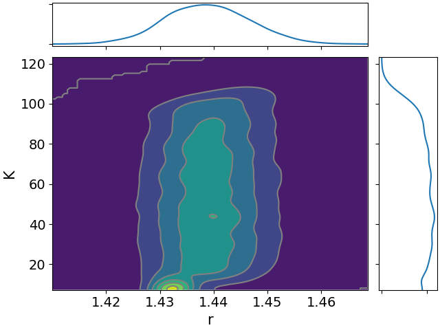
Here are the other posteriors:

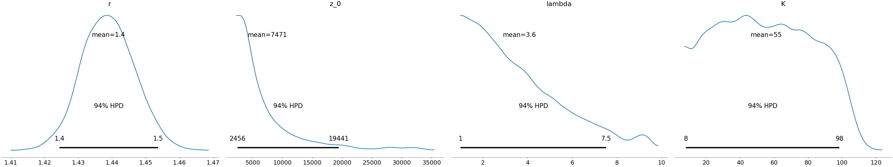
$r$ seems high, maybe implausibly so?

$K$ and $z_0$ are both pretty spread out, but we’ll see they’re inversely correlated, so our estimate for $K z_0$ is more constrained.

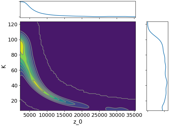
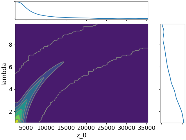
Here are all the joint distributions. One thing of note here is that $K$ is very poorly constrained, but it appears to be strongly correlated with $\lambda$. That suggests that we might be able to constrain $K$ pretty well if we can get a good idea of the time lag between symptom onset and diagnosis.